- AutoEncoder (AE)의 구성에 대해서 설명할 수 있어야 합니다.
- AE의 학습과정을 이해할 수 있다.
- Latent variable의 추상적 개념을 정의할 수 있고,
- 이를 활용하여 기본적인 information retrieval problem를 해결해본다.
- AE의 활용방안에 대해서 생각해볼 수 있다.
AutoEncoder
alibi-detect 라이브러리 사용하면 수월함
https://www.youtube.com/watch?v=RJ4oB6MWTsA&list=PL-xmlFOn6TULrmwkXjRCDAas0ixd_NtyK&index=23
= 디코더로 나온 이미지가 blurry하게 나온다는 단점을 가지고 있다.
==> GAN이 보완
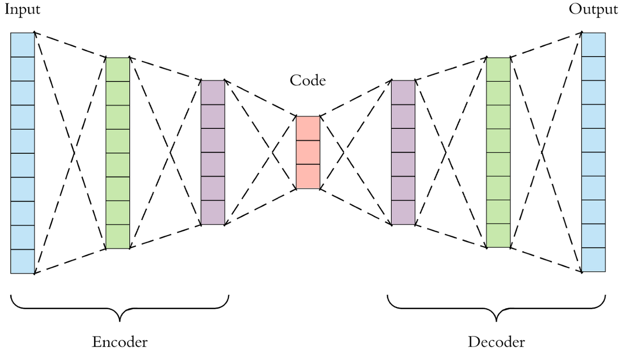
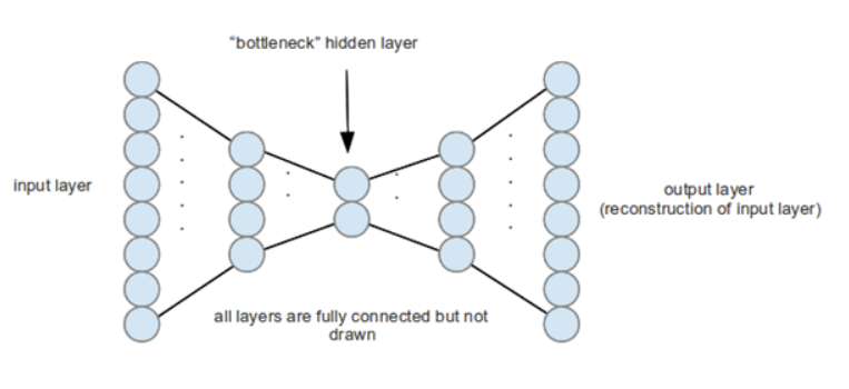
오토인코더(Autoencoders)는 입력데이터 자체를 레이블로 활용하는 학습방식으로, 별도의 레이블이
필요하지 않는 비지도학습 방식입니다.
이는 데이터 코딩(encoding, decoding)을 위해서 원하는 차원만 할당해주면,
자동으로 학습하여 원하는 형태로 데이터의 차원을 축소해주는 신경망의 한 어플리케이션입니다.
차원 축소라기보다 "압축"이라는 표현이 맞다.
차원감소라는 말 대신 “압축”이라는 말을 굳이 사용하는 것은 선형적인 차원감소에서 사용하는 “투영(혹은 정사영)”이
아닌 비선형적인 방식의 차원 감소가 이루어지기 때문
오토 인코더의 목적은 네트워크가 중요한 의미를 갖는 신호 외의 "노이즈"를 제거하도록 훈련함으로써
일반적인 차원 축소 방법(Manifold Learning)론들과 비슷한 목적으로 활용됩니다.
= labeling이 없는 image를 압축하고 복원하면서 특징을 잡아낸다.( 원본data와 차이를 비교해서 이상탐지 )
여기서 코딩된 코드영역을 입력 데이터의 잠재적 표현(Latent representation)이라고 부르게 됩니다.
데이터를 잠재적 표현으로 변경하는 차원축소과정(encoding)과 잠재적 표현에서 다시 데이터로
재구성과정(decoding)은 각각의 가중치들의 연산을 통해서 이뤄지고, 이를 신경망을 통해서 학습합니다.
그리고 학습 과정에서는 인코딩 모델(파라미터)과 디코딩 모델(파라미터)가 동시에 학습이 되지만,
이를 각각의 모델로 구분하여 사용가능
오토인코더를 통하여, 데이터의 노이즈를 제거하도록 학습하면, 노이즈가 제거된 데이터의
특징값을 추출하는 특성값 추출기(Feature extractor)로 활용할 수 있고,
이 모델을 다양한 방식으로 활용할 수 있습니다.
*Encoder = manifold learning
- 어떤 시계열 데이터를 압축해서 표현 ( Down-sampling )
= 특징을 뽑아내는 과정
*Decoder = 생성
- Encoder를 통해 압축된 데이터를 다른 시계열 데이터로 변환 ( Up-sampling )
=> 원래 신호를 재구성하는 방법
Decoder로 Latent Variable을 원래의 Data로 만들어 주게 되면 Label로 다시 input data를
사용할 수 있으므로 지도 학습이 가능해지기 때문에 사용한다.
ex) JPEG 도구는 미디어 파일을 가벼운 이진파일로 압축하여 인코딩하고,
표시할 때 픽셀값을 복원하기 위해 디코딩
앞쪽 데이터에 대한 정확한 예측이 선행되면 뒤에 예측에서도 좋은 결과로 이어지는 경우가 많다.
AutoEncoder 주의사항

그림1은 자동차, 비행기, 새, 강아지를 하나의 1차원 벡터(실수)로 압축한 것이고,
그림3은 2차원의 벡터로 압축한 것
그림1은 무생물과 생물로만 구분이 되겠지만,
그림3은 무생물과 생물 그리고 날 수 있는 것과 아닌것으로 구분이 될 수 있습니다.
이러한 특징때문에 encoder와 decoder의 깊이 및 latent vector의 차원(dimension)을 정교하게 잘 결정해야 합니다.
기본 오토인코더

import matplotlib.pyplot as plt
import numpy as np
import pandas as pd
import tensorflow as tf

from sklearn.metrics import accuracy_score, precision_score, recall_score
from sklearn.model_selection import train_test_split
from tensorflow.keras import layers, losses
from tensorflow.keras.datasets import fashion_mnist
from tensorflow.keras.models import Model

(x_train, _), (x_test, _) = fashion_mnist.load_data()

x_train = x_train.astype('float32') / 255.
x_test = x_test.astype('float32') / 255.

print (x_train.shape) # (60000, 28, 28)
print (x_test.shape) # (10000, 28, 28)

# Code영역의 벡터(= Latent vector)의 수 정의
latent_dim = 64

class Autoencoder(Model):
  def __init__(self, latent_dim):
    super(Autoencoder, self).__init__()
    self.latent_dim = latent_dim
    self.encoder = tf.keras.Sequential([
      layers.Flatten(),
      layers.Dense(latent_dim, activation='relu'),
    ])
    self.decoder = tf.keras.Sequential([
      layers.Dense(784, activation='sigmoid'),
      layers.Reshape((28, 28))
    ])

  def call(self, x):
    encoded = self.encoder(x)
    decoded = self.decoder(encoded)
    return decoded

# decoded된 데이터를 output으로 설정함
autoencoder = Autoencoder(latent_dim)

autoencoder.compile(optimizer='adam', loss=losses.MeanSquaredError())
'''
x_train을 입력 및 대상으로 사용하여 모델을 훈련시킵니다.
encoder는 데이터 세트를 784(28x28) 차원에서 latent 공간으로 압축하는 방법을 배우고
decoder는 원본 이미지를 재구성하는 방법을 배웁니다.
'''

autoencoder.fit(x_train, x_train,
                epochs=10,
                shuffle=True,
                validation_data=(x_test, x_test))

# 학습된 모델을 이용하여 테스트 세트의 이미지를 인코딩 및 디코딩하여 모델을 테스트
encoded_imgs = autoencoder.encoder(x_test).numpy()
decoded_imgs = autoencoder.decoder(encoded_imgs).numpy()

n = 10
plt.figure(figsize=(20, 4))
for i in range(n):
  # display original
  ax = plt.subplot(2, n, i + 1)
  plt.imshow(x_test[i])
  plt.title("original")
  plt.gray()
  ax.get_xaxis().set_visible(False)
  ax.get_yaxis().set_visible(False)

  # display reconstruction
  ax = plt.subplot(2, n, i + 1 + n)
  plt.imshow(decoded_imgs[i])
  plt.title("reconstructed")
  plt.gray()
  ax.get_xaxis().set_visible(False)
  ax.get_yaxis().set_visible(False)
plt.show()
노이즈 제거용 오토인코더
- 가중치의 형태를 CNN형태로 가져온다

x_train = x_train.astype('float32') / 255.
x_test = x_test.astype('float32') / 255.

x_train = x_train[..., tf.newaxis]
x_test = x_test[..., tf.newaxis]

print(x_train.shape) # (60000, 28, 28, 1)

# 노이즈 적용
noise_factor = 0.2
x_train_noisy = x_train + noise_factor * tf.random.normal(shape=x_train.shape)
x_test_noisy = x_test + noise_factor * tf.random.normal(shape=x_test.shape)

x_train_noisy = tf.clip_by_value(x_train_noisy, clip_value_min=0., clip_value_max=1.)
x_test_noisy = tf.clip_by_value(x_test_noisy, clip_value_min=0., clip_value_max=1.)

# 노이즈 이미지 시각화
n = 10
plt.figure(figsize=(20, 2))
for i in range(n):
    ax = plt.subplot(1, n, i + 1)
    plt.title("original + noise")
    plt.imshow(tf.squeeze(x_test_noisy[i]))
    plt.gray()
plt.show()

# CNN의 형태를 갖는 autoencoder 코드
class Denoise(Model):
  def __init__(self):
    super(Denoise, self).__init__()
    self.encoder = tf.keras.Sequential([
      layers.Input(shape=(28, 28, 1)),
      layers.Conv2D(16, (3,3), activation='relu', padding='same', strides=2),
      layers.Conv2D(8, (3,3), activation='relu', padding='same', strides=2)])

    self.decoder = tf.keras.Sequential([
      layers.Conv2DTranspose(8, kernel_size=3, strides=2, activation='relu', padding='same'),
      layers.Conv2DTranspose(16, kernel_size=3, strides=2, activation='relu', padding='same'),
      layers.Conv2D(1, kernel_size=(3,3), activation='sigmoid', padding='same')])

  def call(self, x):
    encoded = self.encoder(x)
    decoded = self.decoder(encoded)
    return decoded

autoencoder = Denoise()

autoencoder.compile(optimizer='adam', loss=losses.MeanSquaredError())
autoencoder.fit(x_train_noisy, x_train,
                epochs=10,
                shuffle=True,
                validation_data=(x_test_noisy, x_test))

# array 변환?
encoded_imgs = autoencoder.encoder(x_test).numpy()
decoded_imgs = autoencoder.decoder(encoded_imgs).numpy()

n = 10
plt.figure(figsize=(20, 4))
for i in range(n):

    # display original + noise
    ax = plt.subplot(2, n, i + 1)
    plt.title("original + noise")
    plt.imshow(tf.squeeze(x_test_noisy[i]))
    plt.gray()
    ax.get_xaxis().set_visible(False)
    ax.get_yaxis().set_visible(False)

    # display reconstruction
    bx = plt.subplot(2, n, i + n + 1)
    plt.title("reconstructed")
    plt.imshow(tf.squeeze(decoded_imgs[i]))
    plt.gray()
    bx.get_xaxis().set_visible(False)
    bx.get_yaxis().set_visible(False)
plt.show()
#########################################################################
from tensorflow.keras.layers import Conv2D, Conv2DTranspose, Dense, Layer, Reshape, InputLayer
from alibi_detect.od import OutlierVAE
from alibi_detect.utils.visualize import plot_instance_score, plot_feature_outlier_image

# alibi_detect VAE
latent_dim = 1024

encoder_net = tf.keras.Sequential([
    InputLayer(input_shape=(64, 64, 3)),
    Conv2D(64, 4, strides=2, padding='same', activation=tf.nn.relu),
    Conv2D(128, 4, strides=2, padding='same', activation=tf.nn.relu),
    Conv2D(512, 4, strides=2, padding='same', activation=tf.nn.relu)
])

decoder_net = tf.keras.Sequential([
    InputLayer(input_shape=(latent_dim,)),
    Dense(4 * 4 * 128),
    Reshape(target_shape=(4, 4, 128)),
    Conv2DTranspose(256, 4, strides=2, padding='same', activation=tf.nn.relu),
    Conv2DTranspose(64, 4, strides=2, padding='same', activation=tf.nn.relu),
    Conv2DTranspose(32, 4, strides=2, padding='same', activation=tf.nn.relu),
    Conv2DTranspose(3, 4, strides=2, padding='same', activation='sigmoid')
])

od = OutlierVAE(
    threshold=.005,
    score_type='mse',
    encoder_net=encoder_net,
    decoder_net=decoder_net,
    latent_dim=latent_dim,
)
이상치 탐지 AnomalyDetector
'''
이 데이터에는 각각 140개의 데이터로 구성된 5,000 개의 심전도(ECG, Electrocardiograms)가
포함되어 있습니다. 각 예제는 '0'(비정상 리듬에 해당) 또는 '1'(정상 리듬에 해당)으로 레이블이
지정된 단순화 된 버전의 데이터 세트를 사용합니다. 비정상적인 리듬을 식별해볼 것입니다.
'''
dataframe = pd.read_csv('http://storage.googleapis.com/download.tensorflow.org/data/ecg.csv', header=None)
raw_data = dataframe.values
dataframe.head()

# data split
# 마지막으로 포함된 레이블을 따로 저장합니다.
labels = raw_data[:, -1]

# 데이터에서는 레이블을 제거해줍니다.
data = raw_data[:, 0:-1]

train_data, test_data, train_labels, test_labels = train_test_split(
    data, labels, test_size=0.2, random_state=21
)

# min-max 알고리즘을 이용하여 정규화합니다.
min_val = tf.reduce_min(train_data)
max_val = tf.reduce_max(train_data)

train_data = (train_data - min_val) / (max_val - min_val)
test_data = (test_data - min_val) / (max_val - min_val)
'''
텐서를 새로운 형태로 캐스팅하는데 사용한다.
부동소수점형에서 정수형으로 바꾼 경우 소수점 버린을 한다.
Boolean형태인 경우 True이면 1, False이면 0을 출력한다.
'''
train_data = tf.cast(train_data, tf.float32)
test_data = tf.cast(test_data, tf.float32)

# True, False data 나눔
train_labels = train_labels.astype(bool)
test_labels = test_labels.astype(bool)

normal_train_data = train_data[train_labels]
normal_test_data = test_data[test_labels]

anomalous_train_data = train_data[~train_labels]
anomalous_test_data = test_data[~test_labels]

# AutoEncoder
class AnomalyDetector(Model):
  def __init__(self):
    super(AnomalyDetector, self).__init__()
    self.encoder = tf.keras.Sequential([
      layers.Dense(32, activation="relu"),
      layers.Dense(16, activation="relu"),
      layers.Dense(8, activation="relu")])

    self.decoder = tf.keras.Sequential([
      layers.Dense(16, activation="relu"),
      layers.Dense(32, activation="relu"),
      layers.Dense(140, activation="sigmoid")])

  def call(self, x):
    encoded = self.encoder(x)
    decoded = self.decoder(encoded)
    return decoded

autoencoder = AnomalyDetector()
# metric은 따로 지정 x
autoencoder.compile(optimizer='adam', loss='mae')

# 정상 ECG 만 사용하여 훈련하고, 테스트 용도에서는 정상과 비정상이 섞인 상태를 평가
history = autoencoder.fit(normal_train_data, normal_train_data,
          epochs=20,
          batch_size=512,
          validation_data=(test_data, test_data),
          shuffle=True)
'''
학습 세트에서 일반 ECG, 오토 인코더에 의해 인코딩 및 디코딩 된 후의 재구성 및 재구성 오류
'''
# 정상 시각화 normal_test_data
encoded_imgs = autoencoder.encoder(normal_test_data).numpy()
decoded_imgs = autoencoder.decoder(encoded_imgs).numpy()

plt.plot(normal_test_data[0],'b')
plt.plot(decoded_imgs[0],'r')
plt.fill_between(np.arange(140), decoded_imgs[0], normal_test_data[0], color='lightcoral' )
plt.legend(labels=["Input", "Reconstruction", "Error"])
plt.show()

# 비정상 시각화 anomalous_test_data
encoded_imgs = autoencoder.encoder(anomalous_test_data).numpy()
decoded_imgs = autoencoder.decoder(encoded_imgs).numpy()

plt.plot(anomalous_test_data[0],'b')
plt.plot(decoded_imgs[0],'r')
plt.fill_between(np.arange(140), decoded_imgs[0], anomalous_test_data[0], color='lightcoral' )
plt.legend(labels=["Input", "Reconstruction", "Error"])
plt.show()

# 이상현상 탐지해보기 = Threshold
'''
재구성 손실이 고정 임계 값보다 큰지 여부를 계산하여 이상을 감지
훈련 세트의 정상 예제에 대한 평균 오차(MAE)를 계산 한 다음 재구성 오차가 훈련 세트의
표준 편차보다큰 경우 향후 예제를 비정상적인 것으로 분류
'''

# 훈련 세트의 정상 ECG에 대한 재구성 오류
reconstructions = autoencoder.predict(normal_train_data)
train_loss = tf.keras.losses.mae(reconstructions, normal_train_data)

plt.hist(train_loss, bins=50)
plt.xlabel("Train loss")
plt.ylabel("No of examples")
plt.show()

# Threshold 설정
'''
평균보다 1SD(1 표준편차만큼)가 높은 임계 값을 선택합니다.
(참고로 통계 수준에서 2SD를 벗어나게 되면, 95%의 신뢰구간을 벗어나는 것을 의미합니다)
'''
threshold = np.mean(train_loss) + np.std(train_loss)
print("Threshold: ", threshold) # Threshold:  0.032173388

# 정상, 비정상으로 나눈 데이터가 아닌 test data
def predict(model, data, threshold):
  reconstructions = model(data) # = model.predict(data)
  loss = tf.keras.losses.mae(reconstructions, data)
  return tf.math.less(loss, threshold)
  '''
  (x <y)의 진리 값을 요소 단위로 반환
  x = tf.constant([5, 4, 6])
  y = tf.constant([5])
  tf.math.less(x, y) ==> [False, True, False]
  '''

def print_stats(predictions, labels):
  print("Accuracy = {}".format(accuracy_score(labels, preds)))
  print("Precision = {}".format(precision_score(labels, preds)))
  print("Recall = {}".format(recall_score(labels, preds)))

preds = predict(autoencoder, test_data, threshold)
print_stats(preds, test_labels)
'''
Accuracy = 0.944
Precision = 0.9921875
Recall = 0.9071428571428571
'''

*Manifold
*정의
공간상에 데이터들을 표현하면 각 데이터들은 점의 형태로 찍혀질 것입니다.
매니폴드는 이런 점들을 최대한 에러 없이 아우를 수 있는 서브 스페이스라고 정의할 수 있습니다
*목적
Encoder에서는 Mainfold 가정을 통해 Input Data의 고차원 데이터는 희박한 밀도를 가지고 있으므로
저차원의 데이터로 만들어서 원래의 데이터를 잘 설명하는 Manifold를 찾는 것이 목적이다.
- 고차원에서 저차원을 차원을 축소하게 되면 어쨋든 그만큼의 loss가 발생하게 되고 데이터의
특징을 잘 표현할 수 없다.
먼저 차원의 저주가 무엇인지 알아보자
차원의 저주는 Data의 개수는 별로 없는데 이를 설명하려고 하는 변수의 차원은 클 때 일어난다.
오토인코더의 가장 중요한 기능 중의 하나는 바로 매니폴드(manifold)를 학습한다는 것
* 매니폴드 학습을 통한(차원축소) 결과는 4가지 용도로 사용된다.(=역할)
- 데이터 압축
- 데이터 시각화
- 차원의 저주 피하기
- 유용한 특징(feature) 추출하기
출처: https://junstar92.tistory.com/157 [별준 코딩]
학습이 완료된 후에도 일반적으로 입력과 완벽히 똑같은 출력을 만들 수는 없겠지만,
매우 근사한 수치로 복제 Loss function에서 입력과 출력의 차이를 이용하기 때문에 출력은 입력과
최대한 근사하게 만들기 위해서 Latent representation 으로 encoding하고,
다시 data로 decoding하면서 이 latent는 데이터의 정보량이 많은 부분 or 대표적인 속성을 우선학습하게 된다.
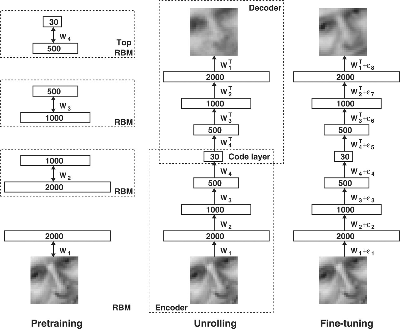
Stacked AE
- “뉴럴네트워크의 층이 깊다”정도에서 끝나는 것이 아니라, “층이 깊어질 때 어떤 좋은 효과가 있는가”에 있다.
뉴럴네트워크는 훈련이 잘 되었다고 가정했을 때, input에 가까운 layer에서는 단순한 pattern에 대한 feature를 추출하는 반면 층이 input에서 멀어질 수록(즉, 깊어질 수록) 더 추상적인 개념에 대해 학습하고 추상적인 feature를 추출할 수 있게 된다고 알려져 있다.
-AE도 hidden layer를 여러 개 쌓아서 구현할 수 있는데 이것을 Stacked AE라고 부른다.
hidden layer가 많을 수록 계속해서 차원을 줄여가는 구조가 된다.
Stacked AE = 계속해서 차원을 줄여가면서 가장 압축된 feature를 얻기 위함이다.
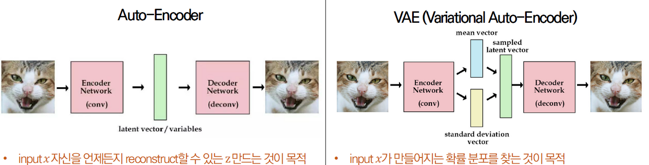
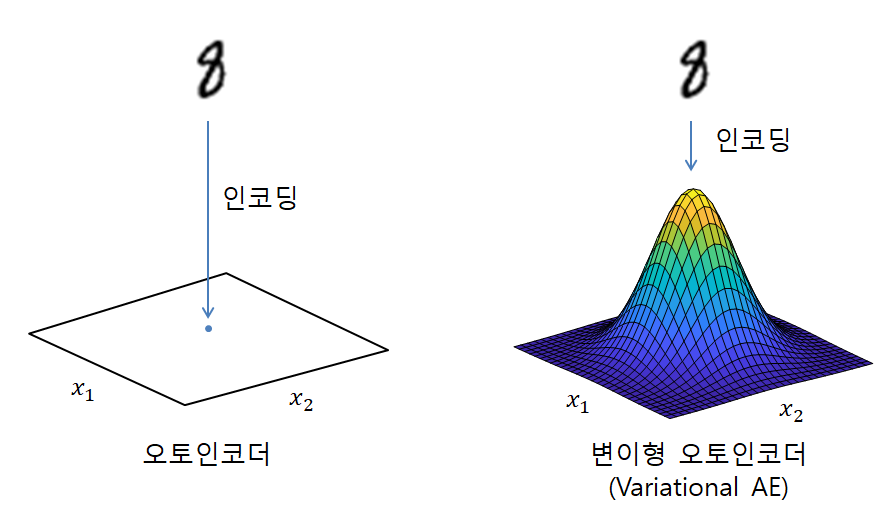
AE vs VAE
AE는
1. 추출된 특징 latent vector를 특정 숫자값을 나타냄
2. Over fitting을 유발
3. Over fitting이 발생하면 한 데이터에 해당하는 latent vector가 한 개만 존재하고, 학습 중에 나타나지 않은 압축 latent vector 에 대해서는 decoder가 전혀 엉뚱한 데이터로 복원하게됨.
Auto Encoder는 본적없는 새로운 데이터를 생성하는 생성 모델로서는 사용이 불가능
만약 데이터의 latent vector 들이 적절한 차원에 적절하게 분포되어 있다면??
VAE는
1.가우시안 확률 분포에 기반한 확률값 (값의 범위)으로 나타냄(= 분포)

<이상치탐지>
GitHub - KerasKorea/KEKOxTutorial: 전 세계의 멋진 케라스 문서 및 튜토리얼을 한글화하여 케라스x코리아
전 세계의 멋진 케라스 문서 및 튜토리얼을 한글화하여 케라스x코리아를 널리널리 이롭게합니다. - GitHub - KerasKorea/KEKOxTutorial: 전 세계의 멋진 케라스 문서 및 튜토리얼을 한글화하여 케라스x코
github.com
'Deep Learning, DL > Computer Vision' 카테고리의 다른 글
| CNN의 기본 과정 정리 (0) | 2022.01.08 |
|---|---|
| 전이학습 (Transfer Learning), 데이터 증강(Augmentation) (0) | 2022.01.08 |
| Generative Adversarial Networks, GAN (0) | 2021.08.29 |
| Image Segmentation(FCN, U-Net) (0) | 2021.08.28 |
| Convolutional Neural Networks, CNN / window? (0) | 2021.08.28 |


댓글